Nonlinear canonical correlation analysis forecasts of the tropical Pacific sea surface temperatures

Aiming Wu and William W. Hsieh

The nonlinear canonical correlation analysis (NLCCA), developed by Hsieh (2000) using a neural network (NN) approach, has been applied to study the nonlinear relation between the tropical Pacific sea level pressure (SLP) and sea surface temperature (SST) fields (Hsieh, 2001), as well as between the wind stress and SST fields (Wu and Hsieh, 2002). Here the NLCCA model is used for the seasonal forecasts of the tropical Pacific SST from the SLP.

The monthly tropical Pacific SLP data (COADS, Woodruff et al. 1987) and the monthly tropical Pacific SST data (Smith et al. 1996) had their seasonal cycles and linear trends removed, and a 3-month running mean applied. As we are still experimenting with the NLCCA approach, the setup of the present NLCCA model differs from that in an earlier issue (Wu and Hsieh, 2001). Predictands are the 6 leading principal components (PCs) of the SST anomalies (SSTA). Predictors are the 10 leading PCs from the singular spectrum analysis (i.e. extended EOF) of the SLP anomalies with a 9-month lag window. The predictors and predictands are the inputs to the NLCCA model. For cross-validation, 5 different models were built. The first was built without the data from 1950-1959, which was to be used as independent validation (or testing) data. Similarly, each of the other models had a different decade of data left out for independent validation.

Due to local minima problems in finding nonlinear modes, only the leading NLCCA mode was used. From the residual data, the linear CCA was used to extract additional modes. Hence the NLCCA forecasts actually use the leading NLCCA mode plus 4 CCA modes. The CCA model uses 5 CCA modes. Using more modes lead to decreasing forecast skills. Table 1 shows the forecasts skills from the nonlinear approach and from the linear approach. Note that for the Nino3.4 and Nino4 regions, at lead times 9 months or longer, the nonlinear approach was marginally worse than the linear approach, due to local minima problems during the nonlinear optimization.

Table 1. The cross-validated correlation skills and root mean square errors (RMSE, in deg. C) over Nino1+2, Nino3, Nino3.4 and Nino4 areas from forecasts by the CCA and NLCCA models, respectively. Calculations were based on the period of 1950 to 2000.


                   Correlation                             RMSE
    ----------------------------------------------------------------------------
    lead  Nino1+2   Nino3  Nino3.4  Nino4     Nino1+2  Nino3  Nino3.4  Nino4
    ----------------------------------------------------------------------------
       0    0.848   0.928   0.935   0.884       0.57    0.31    0.28    0.27
       3    0.701   0.828   0.859   0.823       0.78    0.47    0.41    0.34
  CCA  6    0.464   0.657   0.722   0.725       1.04    0.67    0.58    0.42
       9    0.423   0.537   0.598   0.627       1.11    0.77    0.68    0.49
      12    0.394   0.483   0.507   0.528       1.19    0.84    0.78    0.56
      15    0.280   0.454   0.488   0.487       1.26    0.85    0.77    0.57
    ----------------------------------------------------------------------------
       0    0.833   0.923   0.935   0.903       0.60    0.32    0.28    0.25
       3    0.727   0.829   0.864   0.845       0.75    0.47    0.40    0.31
 NLCCA 6    0.522   0.668   0.735   0.735       0.97    0.65    0.56    0.41
       9    0.431   0.550   0.597   0.615       1.05    0.74    0.68    0.50
      12    0.439   0.517   0.506   0.509       1.06    0.77    0.76    0.56
      15    0.302   0.466   0.470   0.467       1.14    0.80    0.77    0.58
    ----------------------------------------------------------------------------

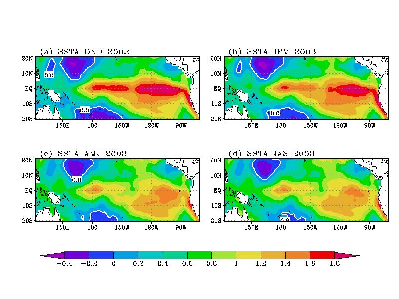
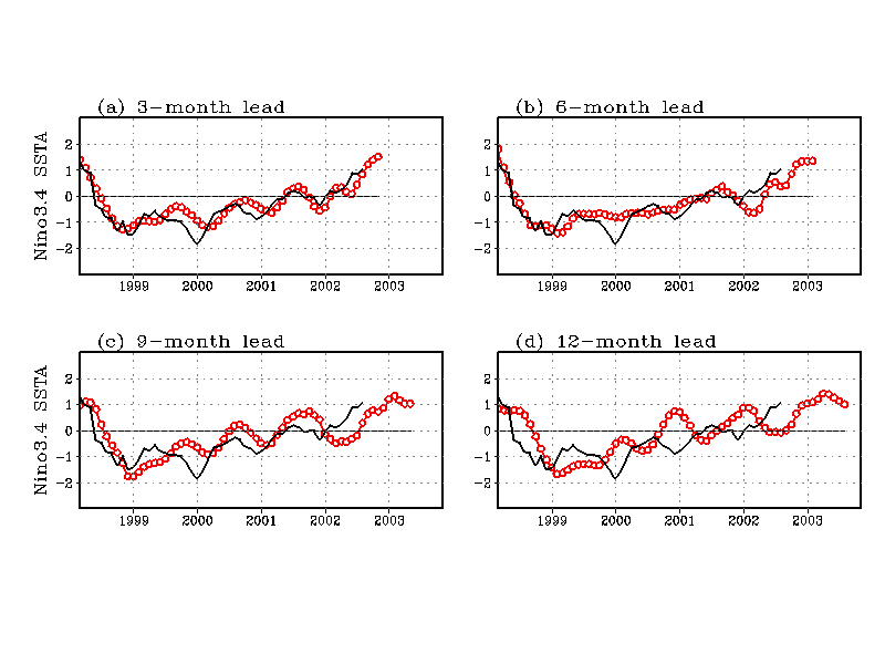
These five models, plus a sixth one trained with data from 1950 till September, 2001, form a 6-member ensemble forecast model. Using data up to the end of August, 2002, forecasts were made with the nonlinear approach. Ensemble-averaged forecasts for the SSTA in the Nino3.4 region at various lead times are shown in Fig.1, showing the development of an El Nino warm event, peaking in early 2003. The forecasted SSTA fields over the tropical Pacific are shown in Fig.2.

Figure 1. The SST anomalies (SSTA) (in degree Celsius) in the Nino3.4 area (170W-120W,5S-5N) predicted by the ensemble-averaged nonlinear model at 3, 6, 9 and 12 months of lead time (circles), with observations denoted by the solid line. Tick marks along the abscissa indicate the January of the given years. (The postscript file of Fig.1 is also available).

Figure 2. SSTA (in degrees Celsius) predicted by the ensemble-averaged nonlinear model at 3, 6, 9 and 12 months of lead time, corresponding to the four consecutive seasons starting with OND (October-December) of 2002. The zero contour is shown as a white curve. (The postscript file of Fig.2 is also available).

References

Hsieh, W.W., 2000. Nonlinear canonical correlation analysis by neural networks. Neural Networks 13: 1095-1105.

Hsieh, W.W., 2001. Nonlinear canonical correlation analysis of the tropical Pacific climate variability using a neural network approach. J. Clim. 14: 2528-2539. (reprint in PDF or preprint in postscript).

Smith, T.M., Reynolds, R.W., Livezey, R.E. and Stokes, D.C., 1996. Reconstruction of historical sea surface temperatures using empirical orthogonal functions. J. Clim. 9: 1403-1420.

Woodruff, S.D., Slutz, R.J., Jenne, R.L. and Steurer, P.M., 1987. A comprehensive ocean-atmosphere data set. Bull. Amer. Meteorol. Soc. 6: 1239-1250.

Wu, A. and W.W. Hsieh, 2001. Forecasting the tropical Pacific sea surface temperatures by nonlinear canonical correlation analysis. Experimental Long Lead Forecast Bull., Sep. 2001.

Wu, A. and Hsieh, W.W., 2002. Nonlinear canonical correlation analysis of the tropical Pacific wind stress and sea surface temperature Clim. Dynam., in press.

Back to [UBC Climate Prediction Group Home Page]